getting-started
getting-started.RmdIntroduction
The ProtPipe package provides downstream proteomics
workflows based on SummarizedExperiment. This vignette uses
a packaged example object so the analysis starts from a ready-to-use
dataset rather than reconstructing the object from raw files.
Setup and Data Loading
First, we load the ProtPipe package.
suppressPackageStartupMessages(library(ProtPipe))
library(SummarizedExperiment)
library(ggplot2) # For plot customization
Load the packaged example object with data(). This
object was created from
EXAMPLES/basic_example_data/iPSC.csv without supplying
external sample metadata, so the only sample annotation present
initially is differentiation_day.
data("protpipe_example_se")
se <- protpipe_example_se

se
#> class: SummarizedExperiment
#> dim: 9119 42
#> metadata(2): creation_method processing_log
#> assays(1): intensities
#> rownames: NULL
#> rowData names(2): PG.ProteinGroups PG.Genes
#> colnames(42): Day0_1 Day0_2 ... Day21_5 Day21_6
#> colData names(1): differentiation_day
colData(se)
#> DataFrame with 42 rows and 1 column
#>         differentiation_day
#>                 <character>
#> Day0_1                 Day0
#> Day0_2                 Day0
#> Day0_3                 Day0
#> Day0_4                 Day0
#> Day0_5                 Day0
#> ...                     ...
#> Day21_2               Day21
#> Day21_3               Day21
#> Day21_4               Day21
#> Day21_5               Day21
#> Day21_6               Day21
Initial Quality Control (QC)
Before normalization and analysis, we should assess the quality of our data.
Protein Counts and Intensity Distributions
We can check the number of proteins identified in each sample and visualize the intensity distributions with boxplots.
# Get the number of identified proteins per sample
ProtPipe::get_pg_counts(se)
#>          Sample Protein_Groups
#> Day0_1   Day0_1           8746
#> Day0_2   Day0_2           8451
#> Day0_3   Day0_3           8571
#> Day0_4   Day0_4           8697
#> Day0_5   Day0_5           8592
#> Day0_6   Day0_6           8433
#> Day28_1 Day28_1           7686
#> Day28_2 Day28_2           7541
#> Day28_3 Day28_3           7305
#> Day28_4 Day28_4           7570
#> Day28_5 Day28_5           7500
#> Day28_6 Day28_6           7631
#> Day03_1 Day03_1           8334
#> Day03_2 Day03_2           8261
#> Day03_3 Day03_3           8193
#> Day03_4 Day03_4           7734
#> Day03_5 Day03_5           8259
#> Day03_6 Day03_6           8229
#> Day07_1 Day07_1           7660
#> Day07_2 Day07_2           7569
#> Day07_3 Day07_3           7939
#> Day07_4 Day07_4           8026
#> Day07_5 Day07_5           7935
#> Day07_6 Day07_6           7755
#> Day10_1 Day10_1           7835
#> Day10_2 Day10_2           7965
#> Day10_3 Day10_3           7663
#> Day10_4 Day10_4           7902
#> Day10_5 Day10_5           7629
#> Day10_6 Day10_6           7724
#> Day14_1 Day14_1           7813
#> Day14_2 Day14_2           7777
#> Day14_3 Day14_3           7827
#> Day14_4 Day14_4           7725
#> Day14_5 Day14_5           7756
#> Day14_6 Day14_6           7653
#> Day21_1 Day21_1           7810
#> Day21_2 Day21_2           7654
#> Day21_3 Day21_3           7815
#> Day21_4 Day21_4           7696
#> Day21_5 Day21_5           7765
#> Day21_6 Day21_6           7771

# Plot the counts for each sample
ProtPipe::plot_pg_counts(se)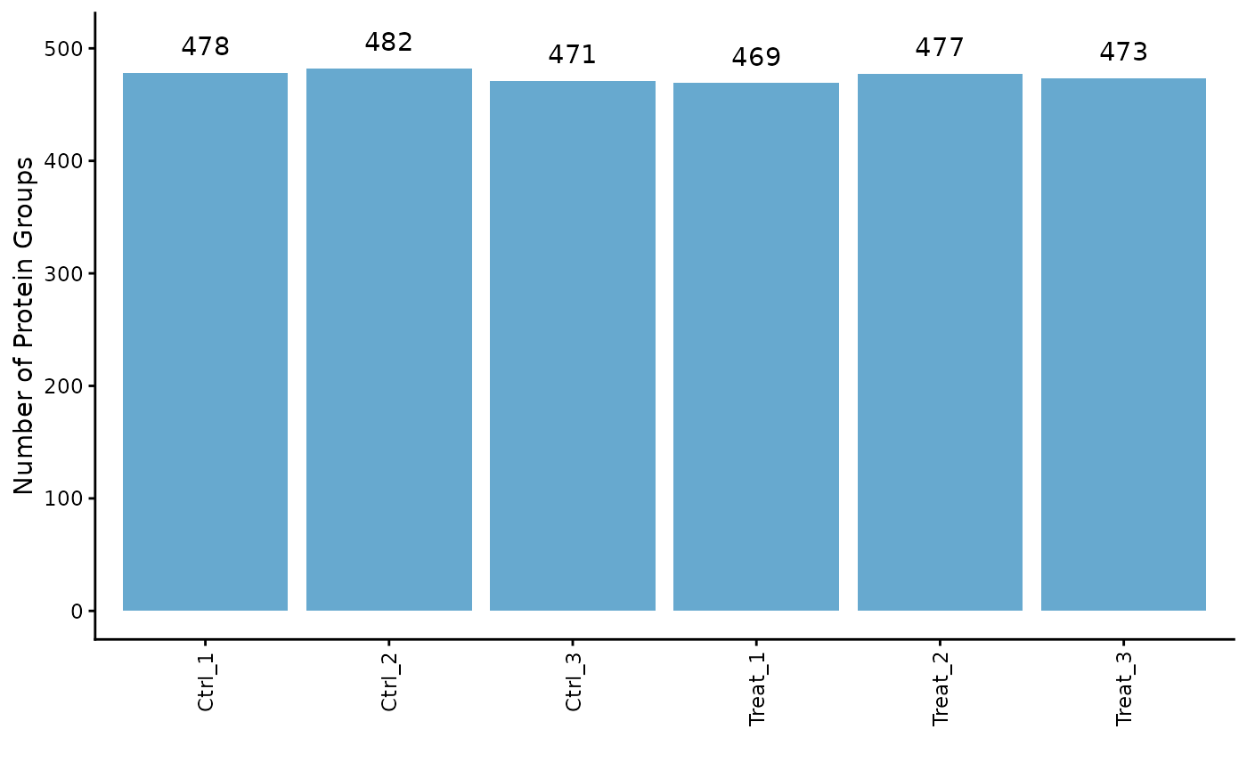
# Plot the intensity distributions for each sample
ProtPipe::plot_pg_intensities(se)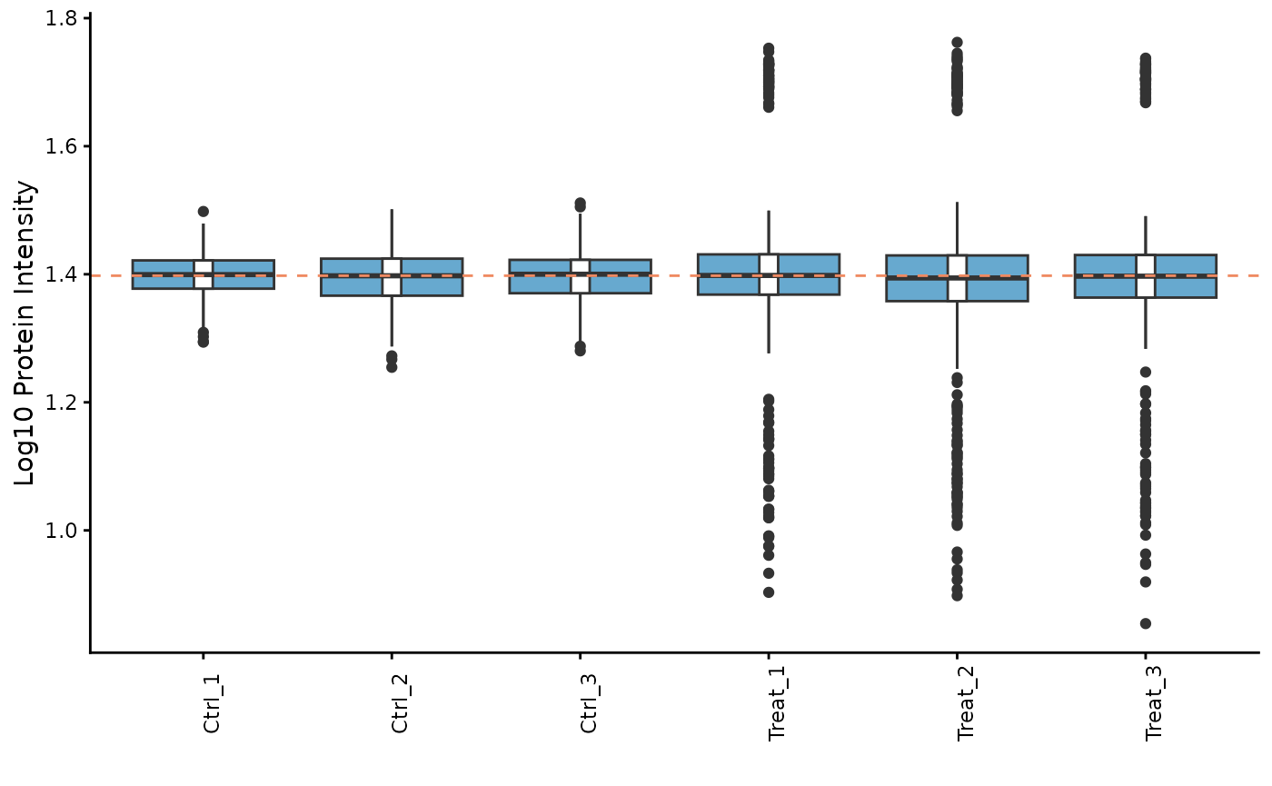 These plots help us identify any samples that behave as strong
outliers.
These plots help us identify any samples that behave as strong
outliers.
Sample Correlation
Next, we can assess the reproducibility between replicates by plotting a correlation heatmap. Samples from the same condition should generally cluster together.
ProtPipe::plot_correlation_heatmap(se)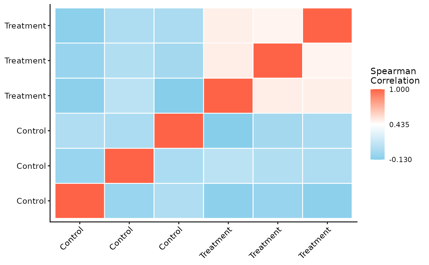
Data Pre-processing
ProtPipe includes functions for common pre-processing
steps like normalization and imputation.
Normalization
Here, we apply median normalization to align the intensity distributions across all samples.
se_normalized <- ProtPipe::median_normalize(se)

# We can re-plot the intensities to see the effect of normalization
ProtPipe::plot_pg_intensities(se_normalized)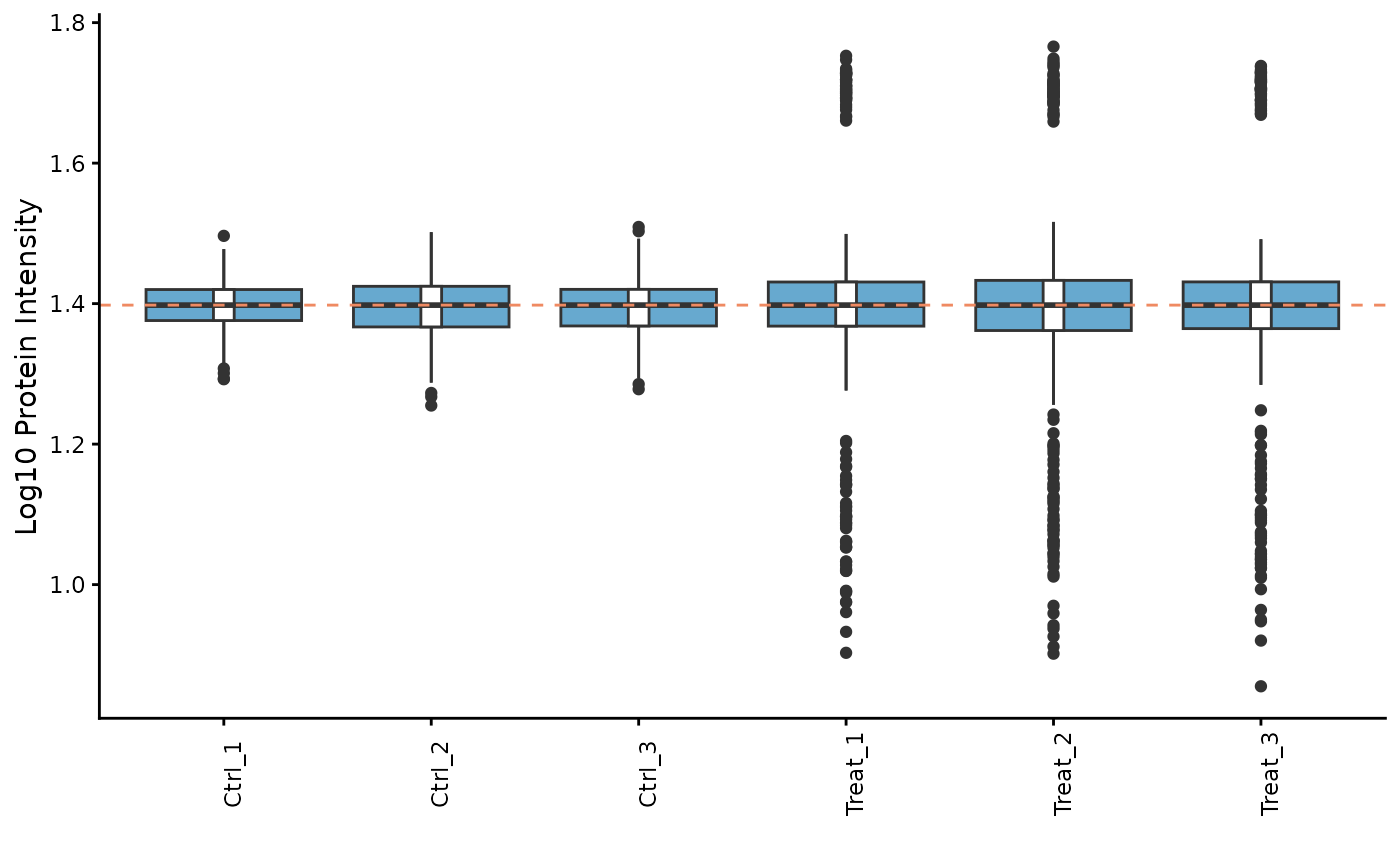
Imputation
Missing values must be handled before many downstream analyses. We will use the “down-shifted normal” (Perseus-like) imputation method. As this is a stochastic method, we set a seed for reproducibility.
set.seed(123) # Set a seed for reproducible imputation
se_imputed <- ProtPipe::impute_left_dist(se_normalized)

# The object should no longer have missing values
any(is.na(assay(se_imputed)))
#> [1] FALSE

# Create a preprocessing report
report <- generate_preprocessing_report(se_imputed)
Downstream Analysis and Visualization
With a clean, complete dataset, we can now explore the relationships between samples and proteins.
Principal Component Analysis (PCA)
PCA is a powerful tool for visualizing the primary sources of variation in the data and assessing sample clustering.
# The plot_pca function is a convenient wrapper that calculates and plots the results
ProtPipe::plot_PCs(se_imputed, condition = "differentiation_day") +
  labs(title = "PCA by time point")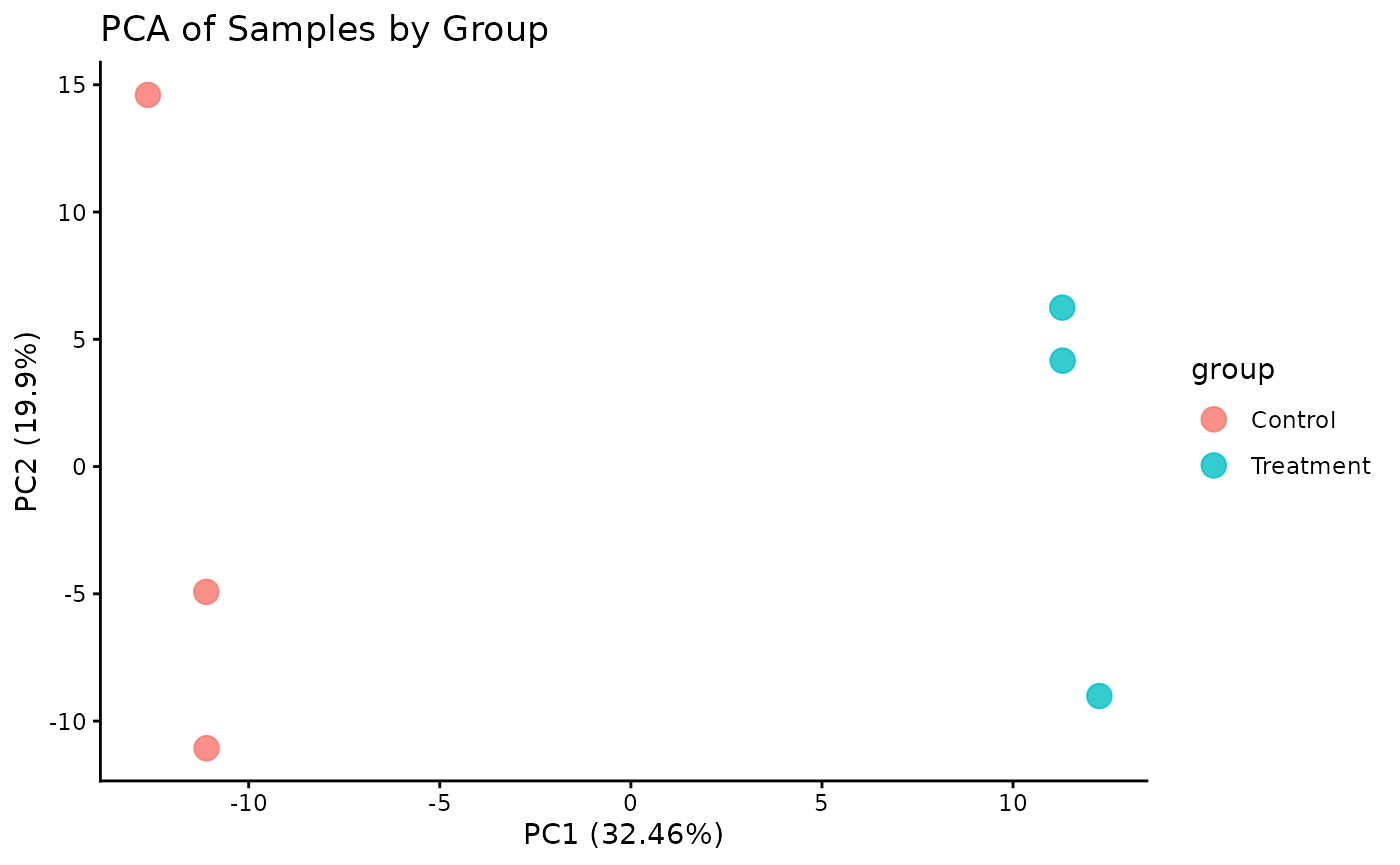
UMAP
Lets plot a UMAP.
# The plot_pca function is a convenient wrapper that calculates and plots the results
ProtPipe::plot_umap(se_imputed, condition = "differentiation_day", neighbors = 6) +
  labs(title = "UMAP by time point")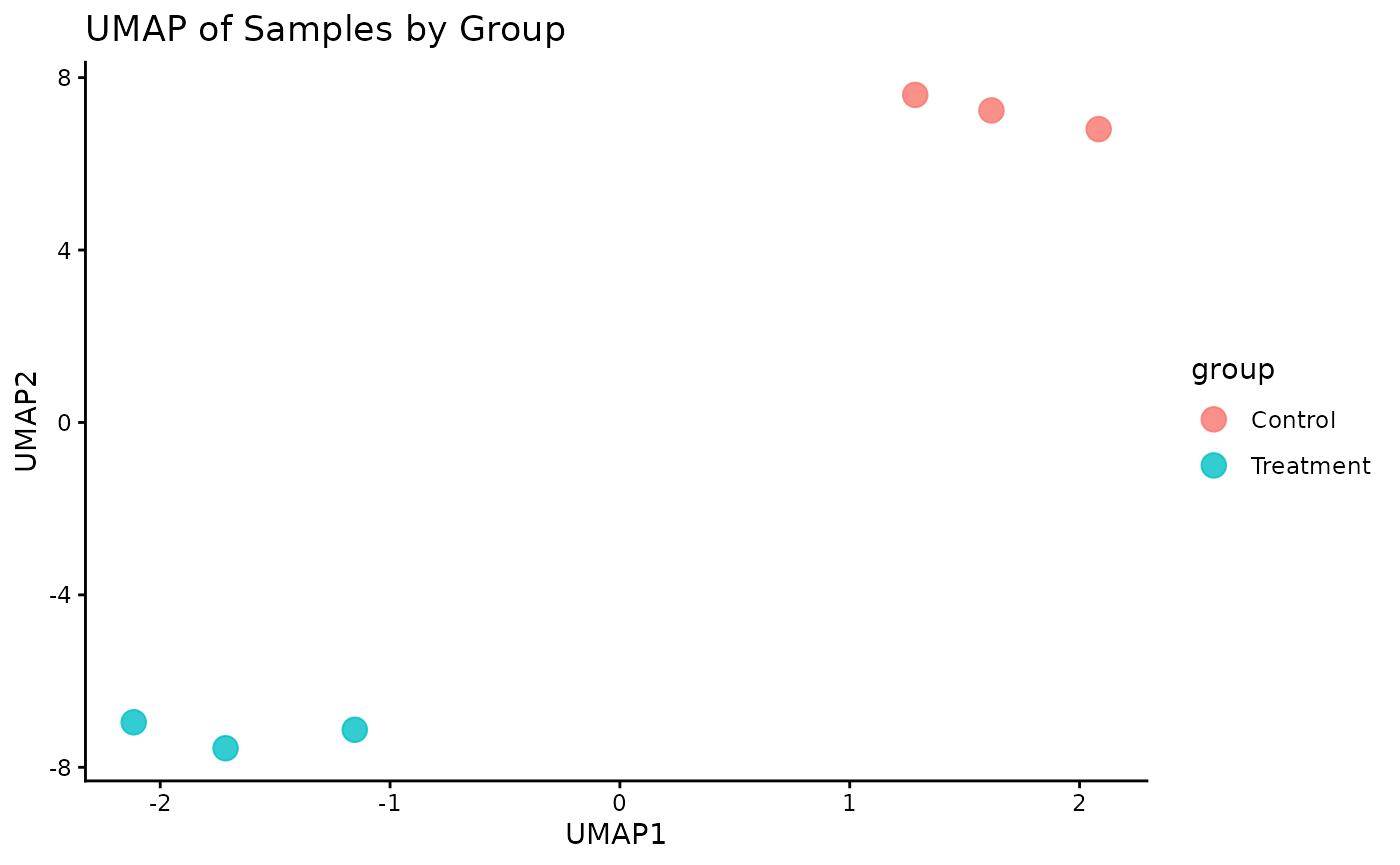
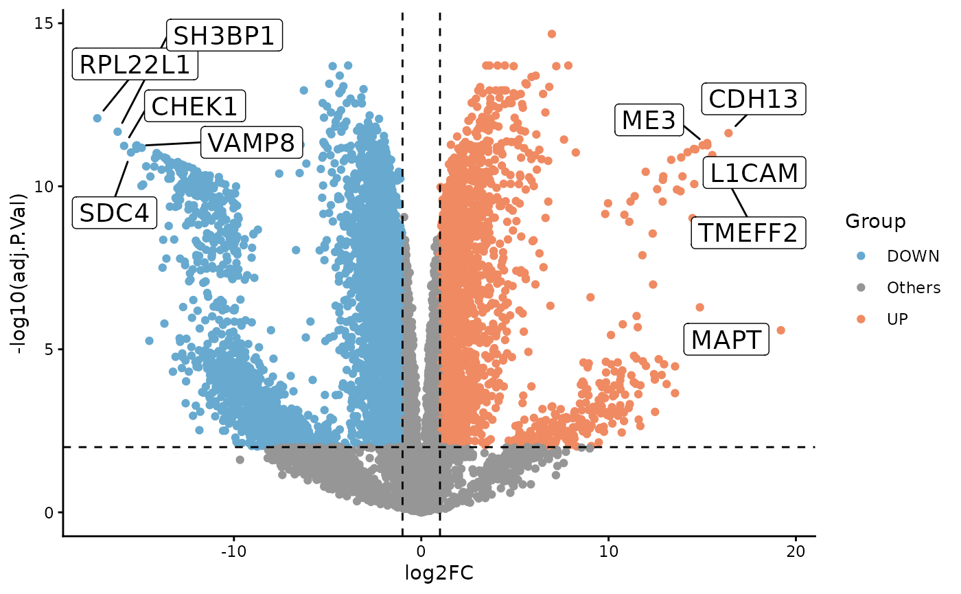
Differential Expression
To illustrate a simple two-group comparison, we compare Day 28 and Day 0 directly with limma.
de <- ProtPipe::do_limma_binary(
  se_imputed,
  condition = "differentiation_day",
  control_group = "Day0",
  treatment_group = "Day28"
)

ProtPipe::plot_volcano(
  de,
  label_col = "PG.Genes"
)
Pathway Analysis
We can perform a simple Gene Ontology enrichment analysis on the differential expression results.
pathways <- ProtPipe::enrich_pathways(
  de,
  gene_col = "PG.Genes",
  source = "go",
  run_gsea = FALSE,
  run_kegg = FALSE
)

pathways$plots$ora_up_dotplot
#> NULL
Protein Expression Heatmap
Finally, we can visualize the expression patterns of the proteins across our samples using a heatmap. The data is automatically Z-scored by row to highlight relative expression changes.
# Plot a heatmap of all proteins with row and column clustering
ProtPipe::plot_proteomics_heatmap(
  se_imputed,
  protmeta_col = "PG.Genes",
  condition = "differentiation_day",
  cluster_rows = TRUE,
  cluster_cols = TRUE
)
#> Condition provided. Summarizing replicates into means...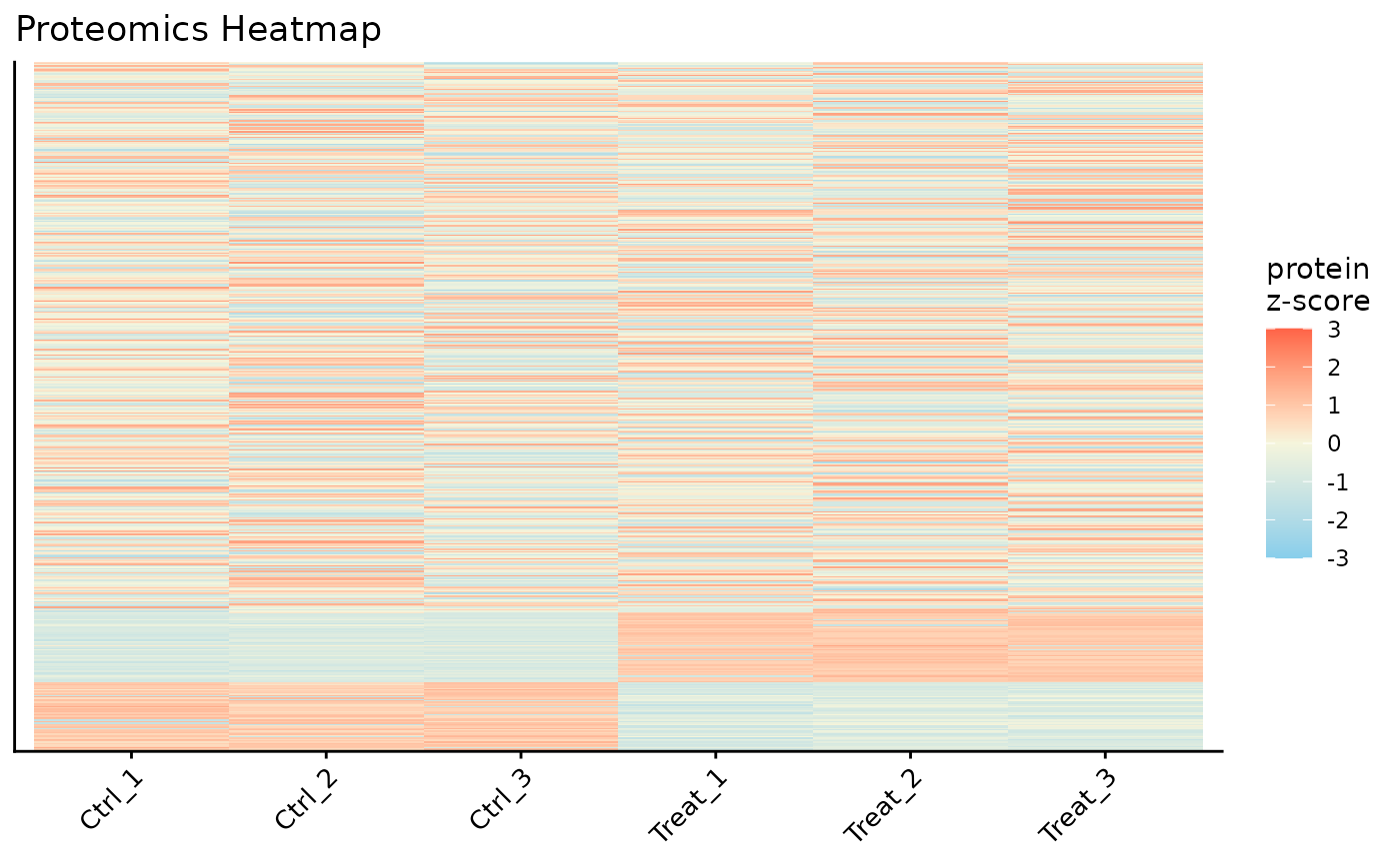
top_genes <- unique(stats::na.omit(de$PG.Genes))[1:4]

ProtPipe::plot_proteomics_heatmap(
  se_imputed,
  protmeta_col = "PG.Genes",
  condition = "differentiation_day",
  genes = top_genes,
  cluster_rows = TRUE,
  cluster_cols = TRUE
)
#> Condition provided. Summarizing replicates into means...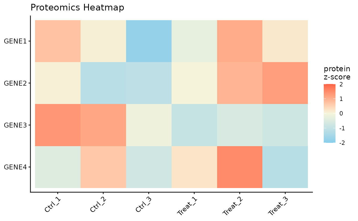
Conclusion
This vignette demonstrated a complete ProtPipe workflow starting from
a packaged SummarizedExperiment. The same pattern extends
to user-supplied objects constructed with create_se().